How to Measure Java Performance - Best Practices and Common Pitfalls

Why the First Java Run Is Misleading

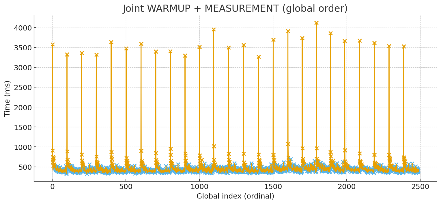
When people say “this Java code takes X ms”, the most important question is: which run? In practice, the very first execution of a Java workload often measures a completely different thing than the next executions. The JVM is still settling in: classes are being loaded, hot methods are being compiled and optimized by the JIT, memory and GC behavior stabilizes, the OS warms up its own caches, and the filesystem page cache starts doing its job. If you time only the first run, you are usually timing initialization + warm-up, not the steady-state performance of your algorithm.

The attached charts show this effect in the clearest possible way. In this particular test, the “cold” executions start around 3.5–4.0 seconds, and after the warm-up the system converges to a steady-state where the median is around ~400 ms, and the typical working level is roughly ~450 ms. That is not a small improvement — it’s almost an order-of-magnitude difference — and it happens without changing the code. It happens because the runtime becomes “hot”.

Why Averages Are Misleading for Java Performance

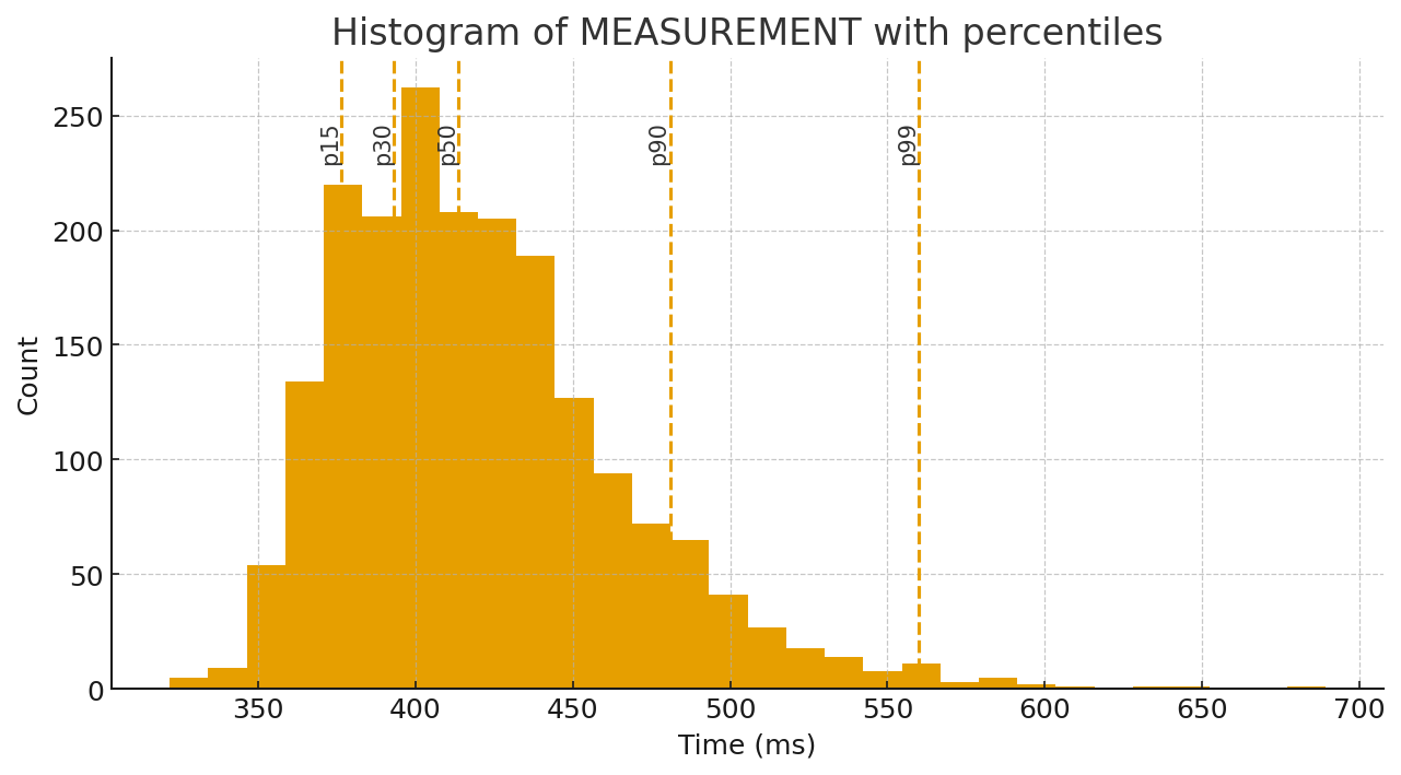
The most common mistake after ignoring warm-up is to summarize everything with a single “average”. Performance timing data rarely looks like a neat bell curve. It tends to be skewed, with occasional spikes from GC, OS scheduling, background I/O, cache misses, and other sources of latency. That’s why looking at the distribution is more honest than trusting a single arithmetic mean. For real-world performance work you want median (p50) as the representative “typical” time, and you also want to watch the tail: p90/p95/p99. Tail latency is where users and production systems often feel pain, and it’s also where regressions can hide if you only track averages.

The histogram with percentiles makes this very tangible: most results cluster around the steady-state band, but there is a visible tail. Those dashed percentile markers tell you far more than one average number ever could.

Using Boxplots to Understand Variability

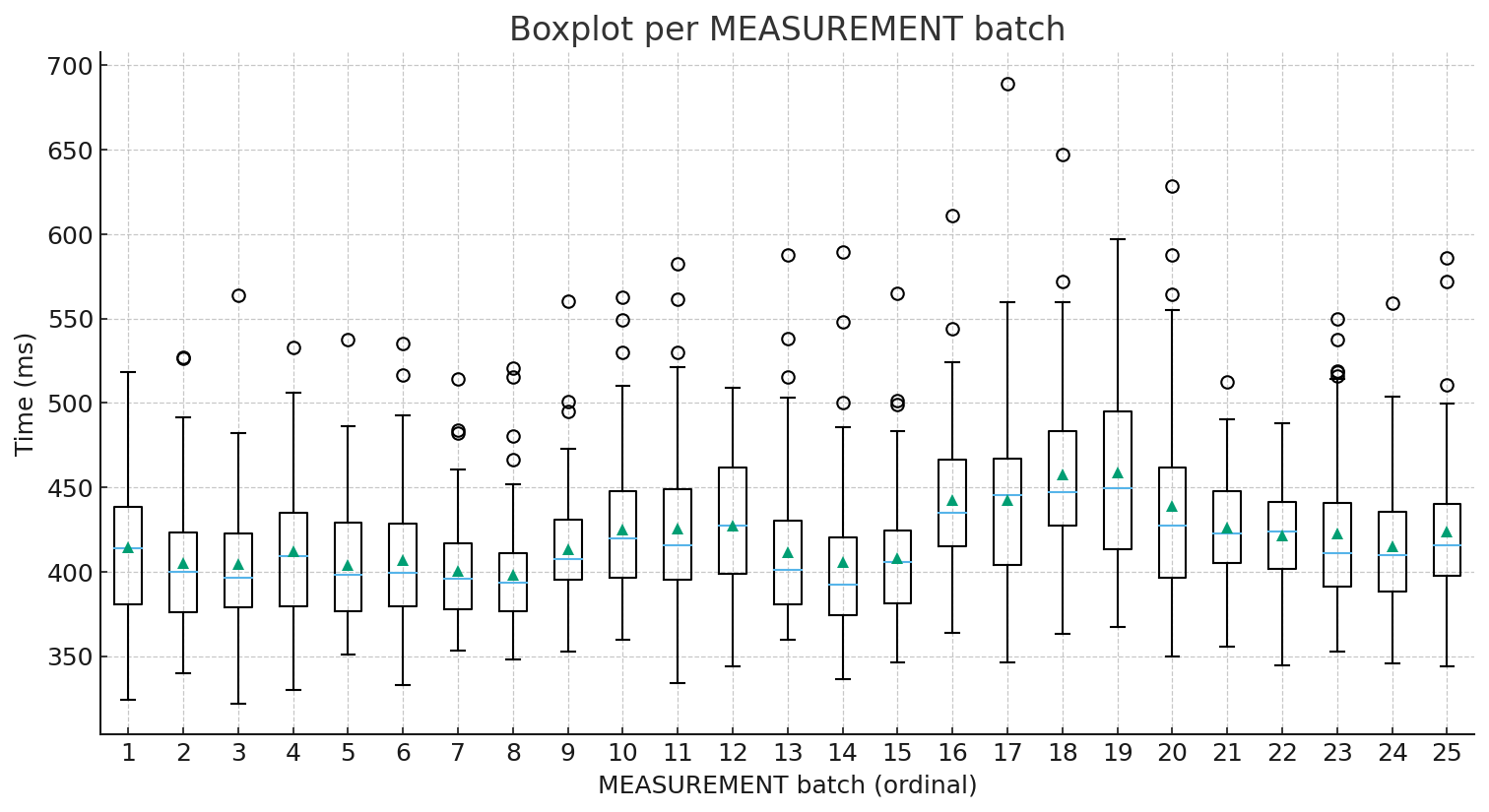
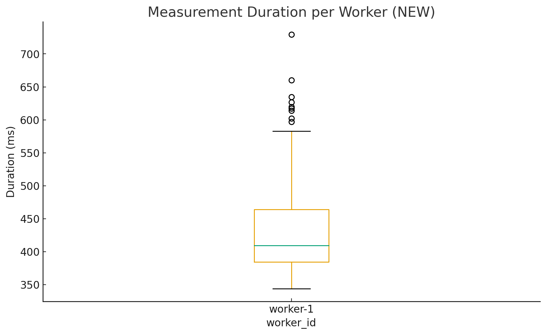
If you want another angle, the batch boxplots (the “candles”) are a great sanity check. The median line inside each box shows where the “typical” run sits, while the spread and outliers show variability. In other words, you see both “how fast” and “how stable”. This is exactly the kind of view you need when you compare builds, JVM versions, GC settings, or small code changes.

Detecting Steady-State Behavior

The moving-average chart adds the story layer: after the first few iterations, the signal settles into a relatively stable region. This is a strong hint that for many practical CI-style checks you don’t need hundreds of runs to get useful numbers — you mainly need to avoid being fooled by cold-start behavior.

Practical Rules for Java Performance Measurement

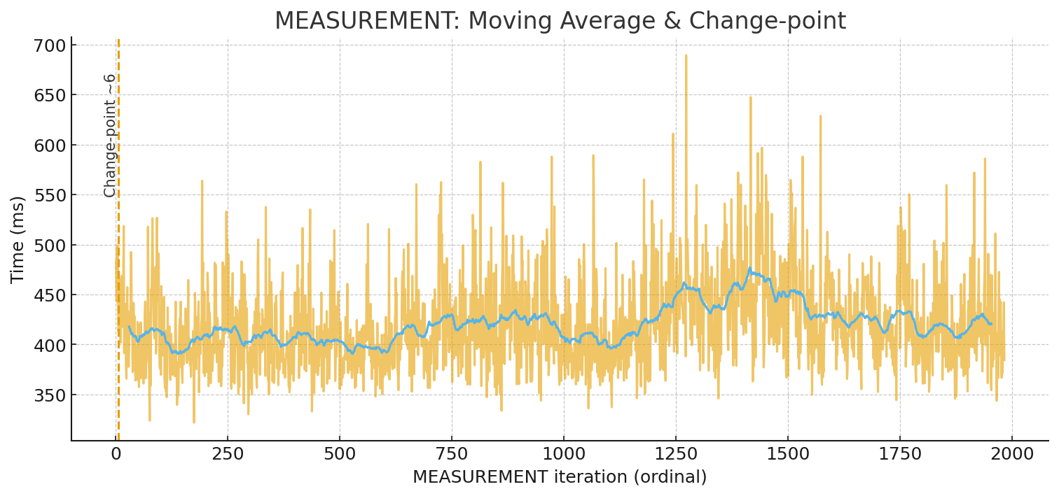
So what should you do in practice? If you’re doing quick comparative measurements (for example, checking whether build A is faster than build B), a simple and effective rule is: run 5–10 iterations, treat the earliest runs as warm-up, and analyze the rest using median and percentiles, not only an average. Your example strongly supports this: the workload reaches its steady state within a handful of cycles, and measuring only once would have produced a completely misleading conclusion.

Why JMH Is Essential for Microbenchmarking

For proper microbenchmarking, the best approach is to use a harness built specifically for JVM realities. The industry-standard tool here is JMH (Java Microbenchmark Harness) from the OpenJDK “Code Tools” project. JMH exists because hand-rolled loops with System.nanoTime() are extremely easy to get wrong on the JVM, especially when the JIT is free to optimize your benchmark code away or transform it in unexpected ways.

Java Warm-Up in Serverless and Microtask Environments

Now zoom out to the world of serverless and micro-tasks. Warm-up is not just an academic concern there — it’s often the concern. When Java runs in environments like AWS Lambda, the cold start can dominate total latency, because the platform may create fresh execution environments under load or after idle periods. That is exactly why “warm-starting” technologies matter.

One important family of solutions is checkpoint/restore. CRaC (Coordinated Restore at Checkpoint) is an OpenJDK project that aims to let you checkpoint a warmed-up JVM process and restore it later, so the application resumes already hot. AWS Lambda’s SnapStart follows a similar spirit: it snapshots an initialized execution environment and restores from that snapshot to reduce latency variability caused by one-time initialization and warm-up. Another widely used direction is GraalVM Native Image, where the application is compiled ahead-of-time into a native executable, often improving startup time and reducing warm-up sensitivity (with trade-offs you need to evaluate for your workload).

Key Takeaways

The key takeaway is simple: if you care about performance numbers, you must respect the lifecycle of the runtime. Java performance is real, but it is also dynamic. Measure it like a dynamic system: run multiple iterations, observe how the distribution behaves, report percentiles, and choose tooling that matches your context — JMH for microbenchmarks, and warm-start technologies like SnapStart/CRaC or AOT approaches like Native Image when cold start dominates.

References (Official Documentation)

• Java Microbenchmark Harness (JMH) — official OpenJDK tool for JVM microbenchmarking
  ( OpenJDK Project, GitHub Repository)

• CRaC (Coordinated Restore at Checkpoint) — OpenJDK project for checkpoint/restore of a warmed-up JVM
  ( Project Page, OpenJDK Wiki)

• AWS Lambda SnapStart for Java — snapshot-based cold start optimization for Java functions
  ( SnapStart Overview, Java Runtime Hooks)

• GraalVM Native Image — ahead-of-time compilation of Java applications into native executables
  ( Official Documentation)