LaTeX Figure rendering | Aspose.TeX for Python

In certain situations, you may need to extract specific content from a LaTeX file as a standalone rendered piece, commonly referred to as a figure, without any connection to the page layout. This could be useful, for example, when creating illustrations for an online publication. Our API allows you to accomplish this. The target formats for rendering figures are PNG and SVG, just like with the LaTeX math formula rendering feature. It is worth noting that LaTeX figure rendering is a more general feature compared to LaTeX math formula rendering.

Rendering a LaTeX figure to PNG

If needed, first take a look at the API reference section for this topic. Similar to formula rendering, we will begin with an example. Here it is:

# Create rendering options setting the image resolution to 150 dpi.
options = PngFigureRendererOptions() 
options.resolution = 150             # Specify the preamble.
options.preamble = r"\usepackage{pict2e}"
# Specify the scaling factor 300%.
options.scale = 3000
# Specify the background color.
options.background_color = Color.white
# Specify the output stream for the log file.
options.log_stream = BytesIO()
# Specify whether to show the terminal output on the console or not.
options.show_terminal = True

# Create the output stream for the figure image.
with open(path.join(Util.output_directory, "text-and-formula.png"), "wb") as stream:
    # Run rendering.
    size = PngFigureRenderer().render(r"""\setlength{\unitlength}{0.8cm}
\begin{picture}(6,5)
\thicklines
\put(1,0.5){\line(2,1){3}} \put(4,2){\line(-2,1){2}} \put(2,3){\line(-2,-5){1}} \put(0.7,0.3){$A$} \put(4.05,1.9){$B$} \put(1.7,2.95){$C$}
\put(3.1,2.5){$a$} \put(1.3,1.7){$b$} \put(2.5,1.05){$c$} \put(0.3,4){$F=\sqrt{s(s-a)(s-b)(s-c)}$} \put(3.5,0.4){$\displaystyle s:=\frac{a+b+c}{2}$}
\end{picture}""", stream, options)

# Show other results.
print(options.error_report)
print()
print(f"Size: {size.width}x{size.height}")

To begin, we create an instance of the LaTeX figure renderer options class, where we simultaneously specify the output image resolution.

Next, we need to specify the preamble. Unlike LaTeX math formula rendering, there is no default preamble for LaTeX figure rendering. Therefore, if you are planning to render graphics created using the pict2e LaTeX package, for example, you will need to specify it in the preamble:

\usepackage{pict2e}

Then we instruct the renderer to scale the output by 300%.

The next option determines the background color. Unlike with math formula rendering, we do not need to specify a foreground color, as we assume that the colors are entirely controlled by the LaTeX code. Similarly, the background color is also controlled by the LaTeX code, so this option is simply provided for convenience.

The following line in the example may not be particularly meaningful. It is simply intended to demonstrate that you have the option to direct the log output to a specific stream.

The final option, ShowTerminal, enables you to control whether the terminal output should be displayed in the console.

The method responsible for rendering the figure is FigureRenderer.render(). It returns the size of the figure in points.

The method accepts a stream as the second argument, which is the stream where the image will be written. We create the stream in the next line.

Finally, we invoke the FigureRenderer.render() method itself, passing the options as the third argument. The LaTeX code of the figure is provided as the first argument.

The last few lines of the example display two pieces of information related to figure rendering - the size of the figure and a brief error report (if there are any errors).

Here is the result of rendering.

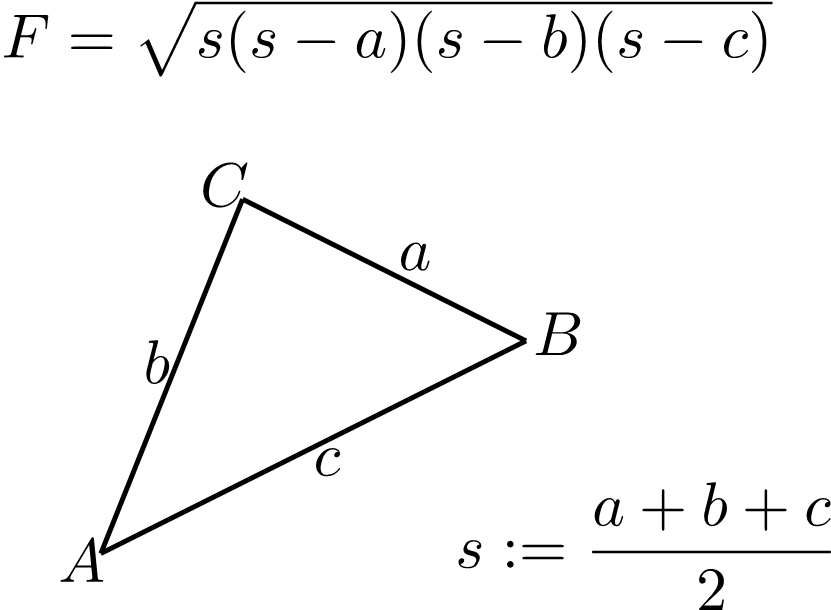
This represents the most general use case for the LaTeX figure rendering feature.

Rendering a LaTeX figure to SVG

Similarly, we can also render a LaTeX figure in SVG format.

# Create rendering options.
options = SvgFigureRendererOptions()
# Specify the preamble.
options.preamble = r"\usepackage{pict2e}"
# Specify the scaling factor 300%.
options.scale = 3000
# Specify the background color.
options.background_color = Color.white
# Specify the output stream for the log file.
options.log_stream = BytesIO()
# Specify whether to show the terminal output on the console or not.
options.show_terminal = True

# Create the output stream for the figure image.
with open(path.join(Util.output_directory, "text-and-formula.svg"), "wb") as stream:
    # Run rendering.
    size = SvgFigureRenderer().render(r"""\setlength{\unitlength}{0.8cm}
\begin{picture}(6,5)
\thicklines
\put(1,0.5){\line(2,1){3}} \put(4,2){\line(-2,1){2}} \put(2,3){\line(-2,-5){1}} \put(0.7,0.3){$A$} \put(4.05,1.9){$B$} \put(1.7,2.95){$C$}
\put(3.1,2.5){$a$} \put(1.3,1.7){$b$} \put(2.5,1.05){$c$} \put(0.3,4){$F=\sqrt{s(s-a)(s-b)(s-c)}$} \put(3.5,0.4){$\displaystyle s:=\frac{a+b+c}{2}$}
\end{picture}""", stream, options)

# Show other results.
print(options.error_report)
print()
print(f"Size: {size.width}x{size.height}")

The differences are:

• Instead of using the PngFigureRendererOptions class, we utilize the SvgFigureRendererOptions class.
• We do not need to specify the resolution.
• Instead of using the PngFigureRenderer class, we utilize the SvgFigureRenderer class.

Here is the result: