PHP でプレゼンテーションチャートにトレンドラインを追加する

このページの概要

Aspose.Slides for PHP via Java を使用して PowerPoint のチャートにトレンドラインをすばやく追加・カスタマイズし、聴衆を引き付ける実用的なガイドです。

概要

この記事では、Aspose.Slides を使用してプレゼンテーションのチャートにトレンドラインを追加する方法を説明します。チャートの作成方法、チャート系列にトレンドラインを追加する方法、指数、線形、対数、移動平均、多項式、パワーなど、さまざまなトレンドラインのタイプの使用方法を示します。

また、ラインシェイプを挿入してチャートにカスタムラインを追加する方法を説明し、前方および後方のトレンドライン投影値や、PDF や SVG へのエクスポート時、画像としてチャートをレンダリングする際にトレンドラインが保持されるかどうかに関する簡単な FAQ を含んでいます。

トレンドラインの追加

チャート系列にトレンドラインを追加するには TrendlineCollection::add を使用し、タイプは TrendlineType で選択します。この例では、既定のデータでクラスター化された縦棒チャートを作成し、3 つの系列それぞれに 2 本のトレンドラインを追加します。

指数トレンドラインは setDisplayEquation と setDisplayRSquaredValue で式と決定係数を非表示にし、線形トレンドラインは赤色です。対数トレンドラインはカスタムラベル用に addTextFrameForOverriding を使用します。移動平均は 3 データポイントの setPeriod を使用し、カスタム setTrendlineName を設定します。

多項式トレンドラインは次数を 3 に設定し（setOrder）、setForward で 1 カテゴリ前方に伸ばします。パワートレンドラインは setBackward で 1 カテゴリ後方に伸ばします。

use aspose\slides\Presentation;
use aspose\slides\ChartType;
use aspose\slides\TrendlineType;
use aspose\slides\FillType;
use aspose\slides\SaveFormat;

$presentation = new Presentation();
try {
    $slide = $presentation->getSlides()->get_Item(0);

    $chart = $slide->getShapes()->addChart(ChartType::ClusteredColumn, 20, 20, 500, 400);

    $firstSeries = $chart->getChartData()->getSeries()->get_Item(0);

    $exponentialTrendline = $firstSeries->getTrendLines()->add(TrendlineType::Exponential);
    $exponentialTrendline->setDisplayEquation(false);
    $exponentialTrendline->setDisplayRSquaredValue(false);

    $linearTrendline = $firstSeries->getTrendLines()->add(TrendlineType::Linear);
    $linearTrendline->getFormat()->getLine()->getFillFormat()->setFillType(FillType::Solid);
    $linearTrendline->getFormat()->getLine()->getFillFormat()->getSolidFillColor()->setColor(java("java.awt.Color")->RED);

    $secondSeries = $chart->getChartData()->getSeries()->get_Item(1);

    $logarithmicTrendline = $secondSeries->getTrendLines()->add(TrendlineType::Logarithmic);
    $logarithmicTrendline->addTextFrameForOverriding("New log trend line");

    $movingAverageTrendline = $secondSeries->getTrendLines()->add(TrendlineType::MovingAverage);
    $movingAverageTrendline->setPeriod(3);
    $movingAverageTrendline->setTrendlineName("New TrendLine Name");

    $thirdSeries = $chart->getChartData()->getSeries()->get_Item(2);

    $polynomialTrendline = $thirdSeries->getTrendLines()->add(TrendlineType::Polynomial);
    $polynomialTrendline->setForward(1);
    $polynomialTrendline->setOrder(3);

    $powerTrendline = $thirdSeries->getTrendLines()->add(TrendlineType::Power);
    $powerTrendline->setBackward(1);

    $presentation->save("ChartTrendLines.pptx", SaveFormat::Pptx);
} finally {
    $presentation->dispose();
}

トレンドラインの切片の設定

setIntercept を使用して、トレンドラインの Y 値を X = 0 で固定します。この設定は線形、指数、多項式トレンドラインでサポートされています。

たとえば、生産コストモデルでは、非ゼロの生産量の測定値が別のベースラインを示唆していても、既知の固定費 100 から開始する必要がある場合があります。線形トレンドラインの場合、切片を固定すると方程式 y = ax + b が b = 100 に制約され、勾配はその制約の下でデータに合わせてフィットします。これは既にフィットした線を単に移動させるだけではありません。軸交差設定はチャートの軸が交わる位置を制御し、フィットしたトレンドラインの係数を変更するものではありません。

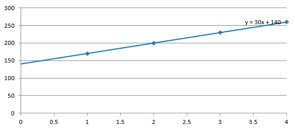
次の例では、生産量が 1 から 4、コストが 170、200、230、260 の散布図（XY）チャートを作成します。デフォルトの自動切片でチャートを保存し、切片を 100 に設定して 2 番目の PPTX を保存します。2 つのファイルは切片設定のみが異なります。トレンドラインは式を表示し、X = 0 まで伸びます。

use aspose\slides\Presentation;
use aspose\slides\ChartType;
use aspose\slides\TrendlineType;
use aspose\slides\SaveFormat;

$presentation = new Presentation();
try {
    $slide = $presentation->getSlides()->get_Item(0);

    $chart = $slide->getShapes()->addChart(ChartType::ScatterWithMarkers, 20, 20, 480, 210);
    $chart->setLegend(false);

    $chart->getChartData()->getSeries()->clear();
    $chart->getChartData()->getCategories()->clear();

    $workbook = $chart->getChartData()->getChartDataWorkbook();
    $workbook->clear(0);

    $nameCell = $workbook->getCell(0, 0, 1, "Production cost");
    $series = $chart->getChartData()->getSeries()->add($nameCell, ChartType::ScatterWithMarkers);
    $costs = [170, 200, 230, 260];

    for ($i = 0; $i < count($costs); $i++) {
        $xCell = $workbook->getCell(0, $i + 1, 0, $i + 1);
        $yCell = $workbook->getCell(0, $i + 1, 1, $costs[$i]);
        $series->getDataPoints()->addDataPointForScatterSeries($xCell, $yCell);
    }

    $trendline = $series->getTrendLines()->add(TrendlineType::Linear);
    $trendline->setDisplayEquation(true);
    $trendline->setBackward(1);

    $presentation->save("AutomaticIntercept.pptx", SaveFormat::Pptx);

    $trendline->setIntercept(100);
    $presentation->save("FixedIntercept.pptx", SaveFormat::Pptx);
} finally {
    $presentation->dispose();
}

自動計算では、これらのデータから y = 30x + 140 が得られます。切片を 100 に設定すると、約 y = 43.33x + 100 となります。ゼロでのフィット値が既知のベースラインと一致しますが、線はすべてのデータポイントを通過しなくなります。

自動切片	切片 100 の固定

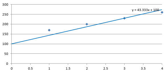両方の画像は同じデータと軸スケールを使用しています。トレンドラインは切片を示すために X = 0 まで伸びています。

デフォルトでは、getIntercept は NaN を返します。これは切片が未指定であることを示し、ゼロではありません。その後、切片はデータから自動的に計算されます。

カスタムラインの追加

カスタムラインは、系列データから計算されたトレンドラインではなく、チャート上に描画されるシェイプです。この例では ShapeCollection::addAutoShape を使用して、チャート上に水平線をスライドに追加します。線の位置はポイント単位のスライド座標で指定され、チャートの左端から開始し、チャートの半分の高さに配置されます。幅はチャートの幅と同じです。getLineFormat で線に単色の赤色を設定します。

use aspose\slides\Presentation;
use aspose\slides\ChartType;
use aspose\slides\FillType;
use aspose\slides\ShapeType;
use aspose\slides\SaveFormat;

$presentation = new Presentation();
try {
    $slide = $presentation->getSlides()->get_Item(0);

    $chart = $slide->getShapes()->addChart(ChartType::ClusteredColumn, 100, 100, 500, 400);

    $lineY = java_values($chart->getY()) + java_values($chart->getHeight()) / 2;
    $line = $slide->getShapes()->addAutoShape(ShapeType::Line, $chart->getX(), $lineY, $chart->getWidth(), 0);
    $line->getLineFormat()->getFillFormat()->setFillType(FillType::Solid);
    $line->getLineFormat()->getFillFormat()->getSolidFillColor()->setColor(java("java.awt.Color")->RED);

    $presentation->save("AddCustomLines.pptx", SaveFormat::Pptx);
} finally {
    $presentation->dispose();
}

FAQ

トレンドラインの「前方」および「後方」は何を意味しますか？

トレンドラインを前方または後方に延長した長さです。散布図（XY）チャートの場合は軸単位で、散布図以外のチャートの場合はカテゴリ数で表されます。負の値は許可されません。

プレゼンテーションを PDF や SVG にエクスポートしたり、スライドを画像としてレンダリングしたりする際に、トレンドラインは保持されますか？

はい。Aspose.Slides はプレゼンテーションを PDF や SVG に変換し、チャートを画像としてレンダリングします。チャートの一部であるトレンドラインはこれらの操作中に保持されます。また、チャート自体の画像を エクスポートするメソッドも用意されています。